Use TEAMFF on Macromolecules
TEAMFF can be used to prepare simulations of molecular systems. In this section, we use macromolecules to see how it works.
If you just start DFF, use File/Recent Project to open the tutorials project. Navigate to the project root folder, right-click, and select Refresh. This will reload all files in this project.
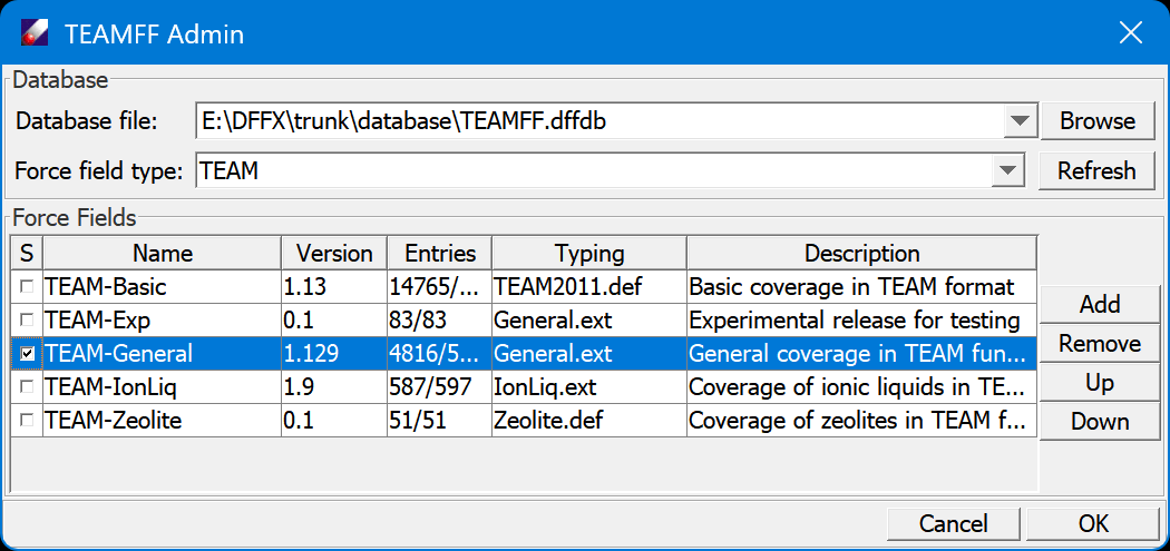
We are using the TEAMFF database in this and following lessons. For exercises, we are using the database come with the tutorials. This is done by use the TEAMFF/Admin command to set up the database. In the dialog, use Browser to find the database provided with the Tutorials at Tutorials/database/TEAMFF.dffdb. The dialog shows force field tables of selected force field type. Select "TEAM" force field type and "TEAM-General" force field to use. Click "OK" to close this dialog.
Working on Polymer and LAMMPS
- In the subfolder tutorialA3_useTEAMFF, there is a polymer mode that has been prebuilt and converted to the MSD format. Double-click on this model to load the structure:
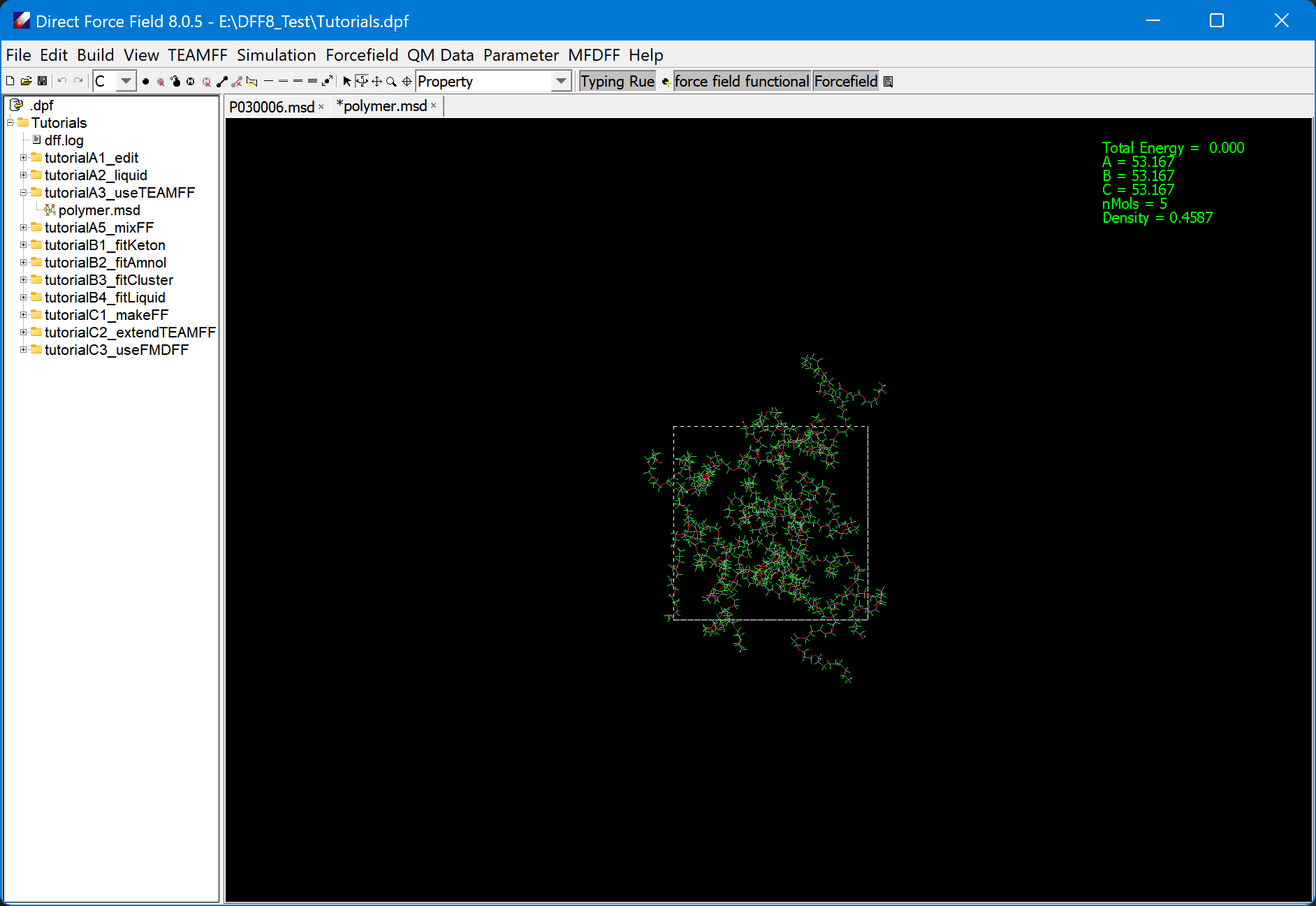
Note that this model has a low density (0.4587), which can be displayed by clicking “Property” in the toolbar. We will compress this model to a density closer to the experimental value.
-
Click TEAMFF/Assign command. This dialog lists the database and force field selected (TEAM-General). The "Output" field lists the file name to be used for the output force field. Unselect Click OK to assign force field parameters. When the job is done, a force field table appears. Review and close the force field table.
-
Select this model, open Edit/Charge Group to assign charge groups, and click Go to assign the charge groups automatically. Leave the "Cross bond charge" to be zero, click Compute command. When the job is completed, the dialog shows 505 charge groups (scroll the display area to view). The largest group contains 7 atoms, the smallest group contains 3 atoms, and all groups have a total charge of zero charge. Click OK to close ths dialog.
-
We now compress the model to a higher density state. Select the model and open Simulation/Molecular Dynamics. Select “NPT”, set “Pressure” to be “1000.0” MPa (very high for a rapid compression), set the “Equilibration steps” to be “100” and “Evaluation steps” to be “200”. Make sure “Screen View” is “On” and click OK.
-
DFF displays density changes during compression. Step 4 can be repeated as needed. Every time a new MD job starts, a subfolder is created for the job. When the system approaches the targeted density (1.5), stop the job. The instantaneous configuration should approximate but not match the target density. To make an exact density of 1.5, we would need to reset the cell edge parameters. The required edge size X1 can be calculated from current edge size X0, current density D0 and target density D1 using the following equation:
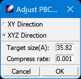
For this system, the target edge size should be 35.82 for a density of 1.5. Select the model, open Build/Adjust PBC, enter the cell edge size, and click OK.
-
Repeat a NVT simulation in DFF to relax the simulation box and verify that the density is indeed correct.
-
Let's submit the simulation to LAMMPS. Selecting the prepared MSD and PPF files from Project Navigator, and clicking Simulation/LAMMPS, which starts the External Simulation window.
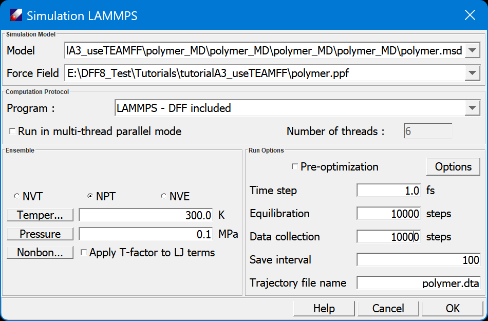
The model and force field files are loaded. Note that the option of “Apply T-factor to LJ terms” is selected, a new force field in which the LJ parameters are scaled according to the applied temperature will be made and used for this job. Select “NVT”, set “Steps” to “1,000” in order to see the results quickly, and note that the “Trajectory file name” is “polymer.dta”. Click OK.
- When the job is finished, a subfolder named as “polymer_LAMMPS” will be created in the Project Navigator. This folder contains the input and output files of this LAMMPS job. Examine the input and output files. Select “polymer.dta” and “polymer.msd” files from the Project Navigator, then click Simulation/Trajectory Viewer to bring up the following dialog box:
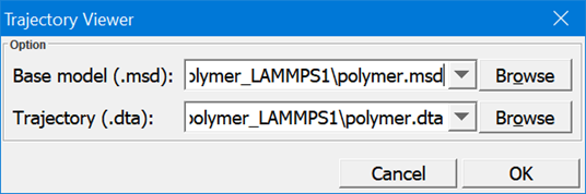
Click OK to start a new window that replays the trajectory. The trajectory is played in a new window, you can use the same viewing options of DFF to translate, rotate, and zoom the models on the trajectory window.
Working On Protein and GROMACS
Models built using external software may need to be modified before assigning a force field. In this lesson, we will work on one example. A protein1.mol2 file is provided with this tutorial. The model does not have hydrogen atoms, so we will assign hydrogen atoms first.
-
Under “tutorials” project, right-click on “tutorialA4_Protein” folder and select add model command in the pulldown menu. In the "Open" dialog, set "Files of type" to “MOL2 Files (*.mol2)” and select “protein1.mol2”. Click Open to load both models.
-
In the Project Navigator, click the newly added model to view it in the main screen. The model does not have hydrogen atoms. Click Add Hydrogen button
 on the tool bar to add hydrogen atoms automatically.
 -
Click TEAMFF/Admin command. Select “AMBER” force field type and “AMBER-General” force field. The, select protein1 in the Project Navigator and click TEAMFF/Assign command. Note that the selected force field, model (protein1), and output force field are listed in the dialog. Click OK to assign force field parameters. When the job is complete, a force field table appears. The force field type is AMBER and the typing rule is “Composed”, which means atom types have been successfully assigned. PREPARE THE MODEL
-
Select “Protein1.msd” from the Project Navigator and click Build/Charge Group. Set “Allow charge crossing a bond” parameter to “0.1” and click Execute. The text area shows the results indicating the largest group has 7 atoms. To define small charge group is essential. The groups do not have to be charge neutral, but the size may be an issue. For example, if the group is too large, GROMACS may fails.
-
Because hydrogen atoms were automatically added, the structure is not relaxed. If the configuration is submitted to GROMACS or LAMMPS, the simulation may fail. Therefore, we should relax this configuration first. To do so, select “Protein1.msd” and open Simulation/Optimization:
Click on “Nonbond Energy”, which opens the following dialog:
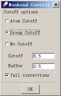
Select “Group Cutoff” and leave other options unchanged. Click OK to close this dialog. Click OK again in the “Optimization” dialog and watch as the energy value drops. When the job is done, the optimized model will be saved to a subfolder named “protein1_OPT”.
-
Now we are ready to submit a job to GROMACS. Click “protein1.msd” from the “protein1_OPT” folder. Make sure the force field is still associated and select Simulation/GROMACS command.
-
Using the default options, set the simulation steps to small numbers (e.g. 1000 steps), and click OK to start the job. The trajectory file will be saved as “protein1.dta”.
-
When the job is complete, a notice will pop up and a subfolder named “protein1_GROMACS” will be placed under the folder in which the job is started. Double-click on the files in this subfolder to see the results of the simulation. Open the “protein1_GROMACS” folder, right-click select Import, set the file type to “GROMACS Trajectory File”, and select “protein1.dta” to load the trajectory file into protein1.dta.
-
Select “protein1.msd” and protein1.dta, then click Simulation/Trajectory Viewer to see the trajectory.